Multiple Regression Analysis

This week we are learning about how to run multiple regression analysis. Regression is one of the most popular statistical techniques that is used to predict a single outcome variable (continuous variable) from multiple independent variables (continuous as well as binary variables). For example, you may want to predict students' academic performance (GPA of a scale from 1-4) from their gender (binary), family income, age, parental education, self-efficacy (all continuous). Having multiple independent variables in a single model allows researchers the confidence to conclude their results while taking into account other factors that may also influence the academic performance variable. As you recall, correlation, ttest, or anova provides results based on a one-on-one relationship (or bivariate relationship). However, these bivariate analyses are also useful for us as they provide a descriptive view to the data.

Now let's look into our data that we used earlier in your ANOVA analysis. Let's say we are interested in predicting academic performance from a few other independent variables such as gender, age, education of mother and father, computer lab used, and parental involvement. Command used for multiple regression is "regress" or "reg" for short. After "reg" is your outcome variable then followed by the rest of your independent variables. Here is how it looks like:  reg rank gender age edumom edudad labuselast parentinvolvement , beta.

However, before we conduct any analysis, we need to check the distribution of our variables being used first. You will need to examine whether or not any of your variables are skewed. Regression analysis is susceptible to outliers. Here is what I would do for the following variables:

sum rank, detail
tab gender
sum age, detail
tab edumom  (you can also do sum edumom, d)
tab edudad (you can also do sum edudad, d)
tab labuselast
sum parentinvolvement, detail

As you know tab will give you percentages to each response and sum, detail gives you skewness value. As you recall from previous class on variable manipulation, the rule of thumb of a normally distributed variable would be a skewness of 1 and lower (nearer to zero is better) and Kurtosis of lower than 3. For more information on skewness and Kurtosis, please refer to this website. All of these variables seem to look okay, except edumom and edudad. See below of the breakdown by each level of education when using tab command:

As you can see only a few fathers having education above high school (only 10 of them) and it is even more disproportional for mothers (only a few of them having high school (3.73%) and above high school education (.60%)). It looks skewed. You can also check it using sum, detail to examine skewness.

As you can see, the skewness of edudad is almost 1 and Kurtosis is exceeding the cut-off point of 3, and the same for edumom. These indicate normal distribution problem.

What can you do?

The best way is to recode these two variables, and then check the skewness again. Let's recode the edudad first, and then you can recode the edumom on your own. As you know, before you recode any variables, it is recommended that you create a new one and use that one, so you can keep your original variable just in case you need to go back later. See the whole process of doing it below:

Those are the 8 steps I would do to recode one variable and to check the skewness of that variable. As you can see, the skewness is reduced to almost zero, and Kurtosis to lower than 3.

Now, it's ready to run our regression analysis:

reg rank gender age edumom_new  edudad_new  labuselast parentinvolvement , beta 

The regression output above shows that the overall regression model with all of these predictors is statistically significant, F(6, 556)=10.16, p<.001, Adjusted R-squared = .09. So first, look at the probability (#1), then R-squared or Adjusted R2 (#2), and if the #1 is significant, then look into individual p values of each predictor (#3). The adjusted R-squared of .09 means that 9% of the variance in the outcome variable is accounted for by the independent variables in the model. Adjusted R2 is preferred when you have many independent variables in your model as it adjusts for the number of variables used in the model. Usually, when you add more variables into the model, R2 tends to increase, so to make sure that variables you include into the model are meaningful (e.g., not just a junk that you throw in), adjusted R2 tells you so. R2 or adjusted R2 also equally indicates effect size, meaning that the larger the R2 values, the larger the effect size, hence more desired. Cohen (1988) indicates that in social science fields, typical effect size tends to be medium.

Based on the regression output above, significant predictors include gender (beta=.23, p<.001), age (beta=.10, p<.05), and parental involvement (beta= -.10, p<.05). Note that if the Prob>F is not significant, then you do not need to mention these significant predictors.

This is an example of how multiple regression table and the write up look like based on the above regression output:

Write Up:

"Table 1 shows that the overall model was significant, F(6, 556)=10.16, p<.001, Adjusted R²=.09. The model explains 9% of variance accounted for by the predictor variables. Factors that predict academic performance include gender (β=.23, p<.001), age (β=.10, p<.05), and parental involvement (β= -.10, p<.05). Specifically, the results suggest that being female, being younger, and having parents who are more involved are significantly associated with better academic performance."

Practice on Your Own

Using the same data above, please predict parental involvement from gender, age, academic performance (rank), education of mother and father, and SES-related variables (electricity, tv, cell, desk, calculator). Your response should include

1. Check to see if your variables are skewed and steps to reduce the skewness
2. Provide commands used at each step
3. Regression table (follow the APA style above)
4. Write up (follow the APA style above)

Note that it is easier and faster for me to read your output if you do the screenshots.

Data Conversion between Software

Today we will learn how to convert data between software: Excel-STATA or SPSS-STATA or vice versa. We will use your Happiness Survey data to practice the conversion.

First of all, let's try converting from Excel -> Stata. Here are the steps: 

1. Open Stata 

2. Click on "File" 

3. Click on "Import"

4. Click on "Excel spreadsheet" 

5. Browse the Excel file you want to import

6. Check the "Import first row as variable names" 

7. OK. 

Here is the screenshot at Step 6:

Then you will see your data in Stata that looks like this: 

You can also Export back your Stata file to Excel file using "File -> Export -> Excel spreadsheet" 

Now let's look at how we can convert this Excel file into SPSS and then to Stata. Here are the steps:

1. Open SPSS software (I still use version 16, very old)

2. Under "File", click on "Open" then "Data"

3. Under "Files of type:" choose "Excel" 

4. Browse the name of your Excel data file, then select it

5. Check the box that says "Read variable names from the first row of data" 

6. Continue 

Here is the screenshot at Step 5: 

Now you have your data in SPSS (converted from Excel), and then you want to convert this SPSS file to Stata. Here are the steps: 

1. Under "File" click on "Save As" 

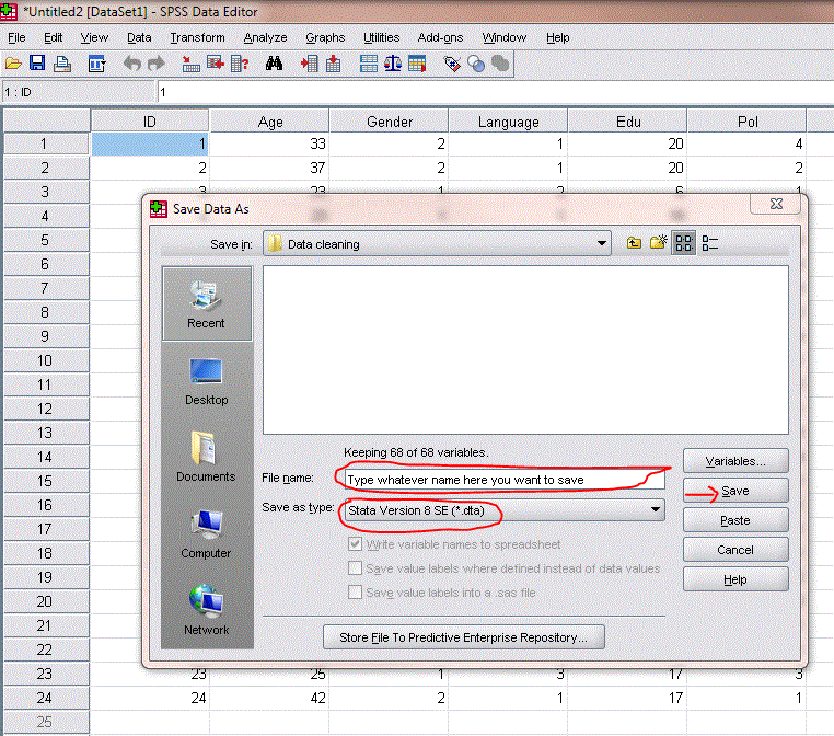
2. Under "Save as type:" choose "Stata" (anyone of them that says Stata) 

3. Under "File name:" type the name you want to save

4. Click on "Save" 

Here is the screenshot at Steps 2-4: 

Analysis of Multiple Response Questions

Multiple response questions are commonly used in a survey questionnaire in which participants could choose more than one answers. For example, students were asked to select the things they like the most about CFC (Caring for Cambodia) schools based on 8 choices: school meal program, beautiful campus, beautiful garden, clean water, toilet, good time with friends, computers, and teachers. In Stata, the analysis of this type is pretty easy and straightforward. First of all, as always, you need to check for the response of the variables being used by using "tab var" command or "codebook var" command.

Before we get into the analysis part, it is important to know how this set of variables is coded. It appears in the questionnaire as just one question though, looking like this:

When you coded this question, it becomes 8 different questions, looking like this in your Stata:

Each question is coded with a numerical value 1 if a respondent answers Yes and 0 if No. For example, if a respondent checks 5 of choices: teacher, food, toilet, computer, garden, then here how it looks like:

If a respondent did not choose any one of the choices, then you can just leave it blank. When you perform an analysis, you can ask Stata to just count all the responses with 1.

Stata does not come with multiple response analysis command which is represented by "mrtab", so we need to install it. The installing process was mentioned during ANOVA lecture when we tried to install "effectsize" command. To install "mrtab" command, type "findit mrtab" in your command box, and a small window will pop up for you to choose a package to install. After you installed it, you can now perform the analysis:

use http://dl.dropboxusercontent.com/u/60032040/mrtab.dta

mrtab cfcteacher- cfcfriend, include response (1) 

So what you see from the output above is that 62.75% of the participants chose good teachers as the thing they like the most about CFC schools. For easy reading of the results, we can ask Stata to sort descendingly for us. We can just add "sort des" after the last option:

mrtab cfcteacher- cfcfriend, include response (1) sort des

Now you can see that the largest number is on the top and the smallest on the bottom.

You can also ask Stata to break it down by school by adding "by (school) col" to the last option:

mrtab cfcteacher- cfcfriend, include response (1) sort des by (school) col

Now the results are broken down by three different schools. Based on the output above, students at Bakong High ranked "good teachers" as the thing they like most about CFC school (72.77%).

You can also request Stata to give us statistical test on chi-square on each individual question by the three schools, and also overall chi-square test of the whole model (all questions together). You can do so by adding "mtest" and "chi2":

mrtab cfcteacher- cfcfriend, include response (1) sort des by (school) col mtest chi2

Look at the last column (chi2/p*). There are two rows of values there, the top one is the chi2 value and the bottom one is the significant value (p). If p value is less than .05, then you can say that there is a significant difference of the response in different schools.

Again, it is always easier to put these values in a graph. Here how it looks like in bar graph:

Let's look at one more example with the same procedure of analysis, using this dataset that you used for your Practice Assignment earlier. Let's look at parental involvement variables (19 of them). The response to these variables range from 1-4. You want to see which involvement variables are the top choices reported by the students in terms of "often" and "most of the time." First of all, you will need to look at the code of any one of the parental involvement variables, since all of them (19) have the same response pattern. For example, I choose involvement item #1 (var: par_invol1):

codebook par_invol1

Now you know that the responses "often" and "most of the time" are 3 and 4. So that means that you want Stata to just include or count the response 3 and 4 in order to know which involvement items rank highest and lowest for "high involvement" category (e.g., 3 and 4 response).

use http://dl.dropboxusercontent.com/u/60032040/assignment1.dta

mrtab par_invol1 - par_invol19, include response (3 4) sort des

As you can see from the Stata output above, the item "My parents reminded me to study hard" ranks highest and "My parents attended meetings at my school" the lowest, for the responses "often" and "most of the time."

If you want to count those who reported just "most of the time" and see which involvement item ranks top, then you can just request Stata to include just "4". It looks like this:

When you count just "most of the time" response (as shown in the above output with number 4 circled in red), involvement item 19 ranks top. This is subjective based on what you want to look into.


Again, you can break it down by gender and you can see if there is a significant difference between male and female students responding to each of the involvement items, for the responses "often" and "most of the time."

mrtab par_invol1 - par_invol19, include response (3 4) sort des by(gender) col mtest

As you can see from the above output by gender, it seems that only involvement item #18 that shows significant difference between males' and females' report on the involvement. It shows that boys are more likely to report that their parents talked about person they admire to them than girls are, χ²(1) = 4.14, p<.05.

You can also make a table out of the above results for easy read. However, since there is no significant difference between gender, then I would not do it.


PRACTICE ON YOUR OWN

Use the question below to answer the following questions:

1. What subject that students like the most? and the least?
2. What subject that students like with the responses from 6-8?
3. Are there any gender differences of each subject (with the response from 6-8)?
4. Please describe your findings in APA format.

use http://dl.dropboxusercontent.com/u/60032040/mrtab.dta

Good luck! 

Correlation

Update (May 12 2014): there is this website that attempts to to build graphs showing correlations between two completely unrelated data. The website's name is Spurious Correlations: Discover a New Correlation. By definition, spurious correlation is a relationship between two variables that are apparent depending on (or with the present of) a third factor. For example, a significant relationship between students dropping out of school and family socioeconomic status depends on students' own academic performance, meaning that family SES alone may not be impacting students' dropping out of school if the students themselves performing well. Therefore, to say that family SES is correlated with student dropout may be misleading or you can say that the relationship between the two variables are spurious. This website updates interesting correlations between two things everyday: http://www.tylervigen.com/

This week we are learning how to conduct correlation analysis. Correlation is a statistical technique that allows you to examine relationship between two variables, both of which are continuous. Correlation does not tell you causal relationship, rather a bi-directional relationship between two variables. Correlation value is expressed by the r value, or a Pearson correlation value. The highest value of r is 1; the higher the value, the stronger the relationship between two variables. The value can be positive or negative; both tell you the direction of the relationship. For example, you may want to know if education of parents is correlated with academic involvement with their children, or education of parents is correlated with age at first school enrollment for their children etc. Correlation gives you an answer in terms of a direction of relationship, and based on the above questions, parents with higher level of education are more likely to be involved in their children's education (positive direction) or parents with higher level of education are less likely to enroll their children late in school (negative). Now let's look at our data as an example. We want to know if education of mother (var name: edumom) is correlated with mother involvement (var name: involvemother). Correlation command is pwcorr. So, pwcorr edumom involvemother, sig (note that IV and DV can be placed anywhere after pwcorr. In ANOVA, DV has to come first after oneway).

use http://dl.dropboxusercontent.com/u/60032040/studentdata2013.dta

pwcorr edumom involvemother, sig

The above output shows that there is a correlation between education of mother and involvement. For your academic paper, you would say that:

"Mother education is positively correlated with mother involvement, r = .10, p<.01. Specifically, the higher levels of mother education, the higher the involvement the mothers have with their children's education."    

You can also request Stata to show you the star on the pair of variables that are significant by using this command option: star (#). You can also request Stata to show you the number of observation of the pair of variables: obs. It looks like this:

pwcorr edumom involvemother, sig obs star(.05) 

The above output shows you see the star on the pair of the variables, with N=804.

Now let's try correlation with more than two variables.

pwcorr edumom edudad involvemother involvefather gender ageenroll rank age, sig obs star(.05) 

Now, let's try to put it into APA style on your own. Things that need to be reported include Pearson r, significant value, and number of observation (N). If there are different numbers of observation, specify the range, from lowest to highest. You don't have to report all of them. That is because by default, Stata uses pairwise deletion method (only pair of missing variables are deleted). Try it! APA style of correlation looks like this:

Correlation examines the relationship between two or more variables separately, meaning that relationship between two variables is independent of other variables (e.g., does not take into account the influence of other variables). It examines between A-B, A-C, or B-C, so A-B is independent of the other two sets. It is just like saying that Income-Education, Education-Age, or Income-Age, but it does not tell you if relationship between income and education depends on age or other variables such as gender. When you have other variables that you want to control for, you need multiple regression. Regression allows you to model your outcome variable based on two or more independent variables, all of which are continuous or dummy in nature. No categorical variables are allowed in regression or correlation.

You con also specify Stata to run for particular group by using "if" command. "if" cannot be placed after a comma. For example,

pwcorr edumom edudad involvemother involvefather ageenroll rank age if gender==1, sig obs star(.05) 

For more information on correlation, you can type "help correlate" in your Stata command box. Or visit: http://www.stata.com/manuals13/rcorrelate.pdf

What if your variables are dichotomous--or more specifically binary? 

Dichotomous variable is the same as categorical variable. Binary variable is a type of dichotomous variable, but with values specifically assigned to both groups as 0 or 1 (e.g., female=0 and male=1). Binary variable is the same as dummy variable where it takes the values of 0 and 1, representing absence or presence of a group.

Let's look at an example below between desk (having a desk at home ("1") or not ("0")) and academic engagement (continuous var) and age (continuous var) of the students. We use command:

pwcorr gender desk engagement age, sig star(.05) 

What we can see based on the above output is that the variable desk is significantly correlated (or associated) with academic engagement (r=.09, p<.01) and age of the students (r= -.11, p<.001). The results specifically suggested that students who have a study desk at home tended to show higher level of academic engagement compared to those who do not have a study desk at home, and students who do not have a desk at home tended to be older compared to those who have a study desk at home.

So how do you read the binary variable "desk"? You know that having a study desk is coded as "1" and not having a study desk is coded as "0". So you look at the sign in front of the correlation (red circles). If it is positive, it represents the "1" which is having a study desk. If it is negative (in the case of age var), it represents the "0" which is not having a study desk.

Now it's your turn to run your own analysis with a binary variable. Use rank and gender and then try to interpret the findings.


PRACTICE ON YOUR OWN

Examine the correlation among the following variables:

rank gender edumom edudad electricity tv cell desk calculator breakfast engagement genderrole

Then, build APA styled table based on the results.

Finally, describe your findings in APA style.

use http://dl.dropboxusercontent.com/u/60032040/studentdata2013.dta

Creating Graphs

This week we are learning different ways of graph building. Reports using graphic illustration helps readers to quickly understand the results of your study. In this class, I am going to show you how to put together a graph in Excel, PowerPoint, or Word, or directly from Stata. There are many categories of graph building including scatter and line plots, range and area plots, bar graphs etc. For more information of graphs, you can type "help graph" in the Stata command box or you can click this link to visit Stata website on graphs. For the purpose of this class, I am going to show you a very simple way of building graphs using bar graphs based on your ANOVA or t-test results.

For example, we are interested in examining the relationship between IT program participation (var name: it) and IT skills (var name: pcskills) of secondary school students in Cambodian schools. IT program participation is a categorical variable with four different groups: (1) those who completed the program, (2) those who passed the enrollment into the program in that year, (3) those who failed to enroll into the program in that year, and (4) those who have never attended the program before. The IT skills variable consists of 15 questions asking them about different IT skills that they know (e.g., do you know how to use Word, save the document, creating graph, creating PPP etc.). The response is yes or no. Those who say yes receives a score of "1" and no of "0". We combined the 15 items together and consider those with higher scores have more IT skills. Cronbach's alpha of this variable is .89. Because the independent variable, IT program participation has 4 groups (more than 2 groups that t-test can handle), we will use ANOVA for this. Thus, oneway pcskills it, t:

Link to data file:  http://dl.dropboxusercontent.com/u/60032040/graphpractice.dta

oneway pcskills it, t

How do you create a bar graph in Word?

First of all, open the Word document, and under Insert, please click on Charts, then choose the default one. The blank Excel sheet will appear for you to input your number. So based on the above Stata output, copy the mean values as circled in red into Excel. Then replace the 4 categories shown in Excel with the 4 categories as shown in this data (the four IT groups) and replace the mean values based on their corresponding categories. Here is how the final Figure looks like based on APA 6th Edition Style:

You can also expand this bar graph by student gender. Here is how it looks like:

oneway pcskills it if gender==0, t
oneway pcskills it if gender==1, t

(Or you can use:
sort gender 
by gender: oneway pcskills it, t)

You can also change the look of the graph to like this: 

PRACTICE ON YOUR OWN 

Create a bar graph based on the following questions: 

use http://dl.dropboxusercontent.com/u/60032040/graphpractice.dta 

1. Is there any significant relationship between lab use (var name: labuselast) and science interests (var name: scienceinterest)? 

2. Is there any significant relationship between lab use (var name: labuselast) and science interests (var name: scienceinterest) for boys and for girls? (hint: run two separate anovas, one for boys and one for girls). 

3. Is students' IT skills (var name: pcskills) associated with education of mother (var name: edumom)? 

4. Is students' IT skills (var name: pcskills) associated with education of father (var name: edudad)? 

Data Analysis: Analysis of Variance (ANOVA)

This week we are learning how to use ANOVA (Analysis of Variance) for your statistical analysis and I want to keep it simple. Let's just focus on oneway ANOVA first. When you are comfortable with it, we can move to twoway ANOVA (e.g., when you have more than one independent variable for one dependent variable). You are using this technique for when your dependent variable is continuous (e.g., age, income, GPA etc.) and your independent variables are categorical (e.g., gender, ethnicity). Fundamentally, you are using ANOVA to find out means (or average) of two or more groups (of your independent variables). Does it sound like another technique that we used from last week? Yes, t-test. T-test does the same thing as ANOVA does. However, t-test can only run a variable that has a maximum of two groups or two levels such as gender (male or female), owning a pet (yes or no), applying for a Ph.D. program (yes or no) etc. When your variable (again, it's your independent variable) exceeds two groups or two levels, then you need ANOVA. Examples would be ethnicity (African American, White, Hispanic, and Asian), types of movie (drama, action, comedy etc.), or year in college if you prefer to use it as a category (freshmen, sophomore, junior, and senior) etc. There are two common commands for ANOVA: (1) anova income gender and (2) oneway income gender, t . I have created a table of type of tests based on the nature of your variables for your easy reference.

Note that the red highlight must be there and if you miss just one thing such as a comma, then it will not run. So you have to be careful about each every detail of your command. This is the reason why I highlighted it in red to ensure that you won't miss anyone of them.

Let's look into this data and run a few ANOVAs. We have questions about students' academic performance (var name is "rank") and mother education and father education. The question is whether parent education plays a key role in student performance. In other words, we can ask if the means of performance (rank) are different by each level of parent education. Here we are using education as a group or categorical variable. We can of course use it as a continuous variable as well, but for the purpose of this practice, let's use it as a group variable. First thing you need to do is to tab parent education (var name is edumom/edudad). So tab edumom and then tab edudad then it will give you percentage of each category of the education level. Why do you need to do the tab first? Because you want to know how does this variable looks like in terms of the response. Here is how it looks like:

Link to data file: http://dl.dropboxusercontent.com/u/60032040/anovapracticedata.dta

tab edumom 
tab edudad

The above table gives you information of percentage of each category of schooling level. Now it is time to run your ANOVAs. We will use the command: oneway rank edumom,t  and oneway rank edudad, t . The ", t" is an option for you to request a table of mean and standard deviation in addition to the statistical values. The variable "rank" is students' academic ranking from 1-50 in which 1 indicates highest performance (again you can do tab rank to see how your this variable's distribution looks like just like you did for edumom and dad).

oneway rank edumom, t 

First of all, look at the circle numbered 1 which shows you the significant level of your analysis. Based on the analysis above, your model is significant (at less than .05 level) and you can say that there is a meaningful difference between mother education and the average score of student performance. Now, it's time to look at the circle numbered 2. We see that the rank mean of mothers with no schooling is the highest (13.5) (meaning that lower performance) and is gradually decreasing with higher levels of education to 5.8 when mothers have above high school education. However, we still do not have any idea if one level is different from another. If there are only two levels, we know right away which one is higher or lower. Now we need a follow up analysis (or post-hoc). There are a few techniques, but we can just use bonferroni test (or bon). Here is now the command would look like, same as above, but adding bon: oneway rank edumom, t bon 

oneway rank edumom, t bon   

What we are looking from the above table is the significant levels of the each comparison (a total of 10 pairs). Let's just look at the pairs that are significant (i.e., less than .05 level). However, all the pairs are above .05 level, but there are two pairs that are marginally significant as shown in the red circles.

No Schooling--Secondary: marginally significant at p=.078
Primary--Secondary: marginally significant at p=.060.

NOW, do your own using father education.
Good luck!

TABLE MAKING

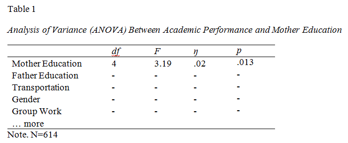
Here is how ANOVA Table should look like in your paper in APA style. Note that ŋ is eta-square or effectsize based on this method. 

REPORTING THE RESULTS 

"Table 1 shows the results based on Analysis of Variance (ANOVA) between mother education and students' academic performance. The results suggest that mother education is significantly associated with students' academic performance, F(4, 609)=3.19, p<.05, ŋ =.02. Post-hoc analysis using Bonferoni method shows that mother with secondary education is significantly different from mothers with no education and mothers with primary education in relations to students' academic performance."  

EFFECT SIZE

What is effect size and how do you obtain it? 

By definition, effect size is a simple way of quantifying the difference between two groups or a way to present the practical significance (rather than statistical significance) of the results. As a convention, effect size based on eta2 (eta-square) of .01 is considered small, .06 medium, and 14 large. The interpretation of effect size should be considered contextually. Coe (2002) argued that "the effectiveness of a particular intervention can only be interpreted in relation to other interventions that seek to produce the same effect. In education, if it could be shown that making a small and inexpensive change would raise academic achievement by an effect size even as little as 0.01, then this could be very significant improvement, particularly if the improvement applied uniformly to all students, and even more so if the effect were cumulative over time." 

Now you will learn how to obtain effect size. The command "oneway" will not work here. We need to use "anova" command this time. Effect size option is not pre-installed in your STATA, so you need to install it. To do so, type findit effectsize . Then a small page popping up looking like this: 

You can click on anyone of them to install. Here is how it looks like: 

It will tells you once the installation has been completed. Now it's time to check your effect size. Type the following command: 

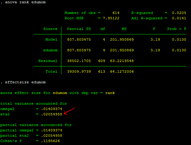
anova rank edumom 

then 

effectsize edumom 

And here is how it looks like: 

So there, you got the effect size. It's .02 as also shown in your ANOVA sample table 1 above. 

R-square also suggests an effect size. You could use that as well. The above R-square is also .0205. The benefit of using effectsize command following the anova command is that you have more effect size options such as omega and Cohen. 

PRACTICE ON YOUR OWN

Using the anovapracticedata (use the same data above: http://dl.dropboxusercontent.com/u/60032040/anovapracticedata.dta), please answer the following questions:

1. Does type of transportation (var name transport) have any relationship with students' academic performance (var name: rank)? What is the effect size?

2. Do students who prefer to work in a group (var name groupwork) perform better academically compared to those who prefer working alone? What is the effect size?

3. Does mother education impact their involvement with their children's education (var name: parentinvolvement)? What is the effect size?

4. Create a question(s) on your own. The independent variable has to have more than two levels/groups.


***Note. This website does a great job in explaining within and between group variances.

Data Analysis: T-TEST

This week we are going to talk about t-test. We use t-test to serve a few purposes but the two main things are comparing means of a continuous variable (e.g., GPA or income) with a categorical variable (e.g., gender or type of university--public vs. private)--that is called "independent group ttest," and comparing means between two continuous variables (e.g, pre-test and post-test)--that is called "paired t-test".

Independent Group T-Test

Research questions for this type of test may include: (1) are there any income differences between male and female employees? (2) Is GPA different by gender? (3) compared to those who have studied abroad, do those who have not earn more salary? (4) do people who went to a private university earn better salary compared to those who went to a public university? etc. Remember that t-test allows only two groups (e.g., male or female; study abroad vs. not study abroad). If you have a variable that has three or more groups (e.g., ethnicity or type of car etc.), then ANOVA (Oneway Analysis of Variance) is appropriate. We will cover this later. Let's look at our studentdata2008 data and try to run a few t-tests. First let's see if there is any difference in GPA between male and female students. The command for it is: ttest gpa, by(sexstud) . Note that the outcome variable (or dependent variable) is placed right after the command ttest and there is a "comma" sign after GPA, followed by "by" and the categorical variable in parenthesis.

Download studentdata2008 for your analysis below:

ttest gpa , by (sexstud) 

The first thing you are looking into at the above figure table is the mean values of female and male. It is clear that female scored higher on their GPA (6.58) compared to male of 5.68. Second, the probability value which in this case the middle one (the two-tailed test**see the notes below: for more information on this, this link to UCLA website is helpful). You are looking at a p value of less than 0.05 so that you can make a conclusion that there is a significant relationship between gender and GPA, specifically, to say that female is more likely to perform better than male. The circle #3 is used for your report write up. There are many ways you can write this up in your paper for your class or publication, but this is what I would write:

"This study seeks to examine the difference between academic performance by students' gender. The results based on an independent group t-test show that female students (M=6.58, SD=.13) tend to perform better than their male counterparts (M=5.68, SD=.14), t(268)=4.67, p<.001."

Note that whenever you report mean, you need to also report standard deviation.

As you recall, last week we also use the command tab/sum to find the mean difference between two groups and it would give the same results to the ttest command. However, the tab/sum command does not give you statistical significance. So for example, if you run tab (sexstud), sum (gpa), you get the following:

tab (sexstud), sum (gpa)

You can see that the tab/sum command above gives you the same mean/sd results, but no statistical significance, and that's when t-test becomes useful.

So now how do you build a table that you can put it in your paper or report? You cannot copy and paste the ttest table above directly to your paper. Here it is a sample that I created for your reference:

If you have more than one variables, you can put them in after the academic performance, but their predictor (or Independent Variable) must be gender, otherwise, you need to create another table for it.

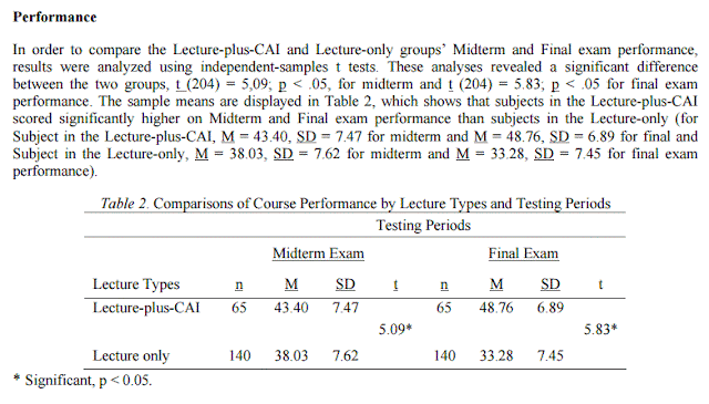
For your real world reference, I included below ttest results from an article published in Educational Technology & Society (pages 170-178) so that you can see the variety of tables are being used. It would be useful later when you become an evaluator of any program.

Paired T-Test 

This type of t-test seeks to answer relationship between two continuous variables that are not independent of one another, meaning that the same participants responded to the two variables at one point or two different times. For example, in my study, I compared involvement by mother and by father as reported by the student. So I have two measures: mother involvement and father involvement. I want to see the average scores of these two measures--which one scores higher? My hypothesis is that mother would have higher level of involvement than father. The command for this test is ttest involvemother==involvefather

Download studentdata2013 for your analysis below:

 ttest involvemother==involvefather 

Based on the above table, you can see that mother scored higher in their involvement with their children (M=2.52, SD=.67) compared to that of father (M=2.46, SD=.73), t(853)=3.37, p<.001.

Now it is your turn to practice your write up based on these above results as well as your APA styled table.

Paired-ttest is also commonly used for comparing scores from two different times, pre-test and post-test that are obtained from the same participants. Look at this report that my colleague, Dr. Scott Plunkett, Professor of Psychology at Cal State, Northridge and I wrote as part of an evaluation for Western Justice Center Foundation located in California, and how the results are reported and how the table is built (link to the report).

and this one:

and here is an excerpt taken from Executive Summary part of the report showing how the results were reported:

Practice on Your Own 

1. Using studentdata2013 data, please compare each involvement score between father and mother. In other words, is involvemom1 different from involvedad1 and so forth for the ten of them. Which one is significant?

2. Using studentdata2013 data, is there a difference between education of mother (edumom) in academic performance (rank) of their children?

3. Using studentdata2013 data, does education of father matter in their children's academic performance (rank)?

4. Using studentdata2013 data, does having electricity at home (electricity) improve students' academic performance (rank)?

5. Using studentdata2013 data, does mother involvement improve academic performance (rank) of their children?

6. Using studentdata2013 data, does father involvement improve academic performance (rank) of their children?

7. Please do not simply paste your outputs, but also add your answer in writing as well.



Note: **, one-tailed test tests just one direction of a relationship; whereas two-tailed test tests both directions (your p-value will need to be divided by two). One-tailed test is more powerful than a two-tailed test, because one-tailed test does not need to be divided--it's just a test for one direction. If you know the direction of your relationship (e.g., females perform better than males), then use a one-tailed test. If you do not know the direction, then use the two-tailed test. If you use a two-tailed test, and want to get a one-tailed result, then just divide the p-value of the two-tailed p-value by 2. In your ttest gpa, by(sexstud) above, your two-tailed test p-value is 0.0000 (the one in the middle). If you divide it by 2, it is still 0.0000 (the one on the right side). To get another one in the left side, you use 1-.0000, and it's 1.0000. To keep it simple, we will just use a two-tailed p-value throughout the class. Also note that usually a two-tailed test is shown by default in any statistical outputs.